COVID-19: A demographic analysis of the trend in Indian cases

Introduction

India in 2019 with population of 1.37 billion and 0.73% death rate experienced about10 million deaths due to various causes. By end of August 2020 India has experienced more than 75,000 deaths due to COVID-19 virus infection cases of 3.3 million.1

Acharya et al. computed a composite index of vulnerability at the state and district levels based on 15 indicators across five domains of socioeconomic, demographic, housing and hygiene, epidemiological, and health system. They utilized a percentile ranking method to compute both domain-specific and overall vulnerability. They found that a number of districts in nine large states of Bihar, Madhya Pradesh, Telangana, Jharkhand, Uttar Pradesh, Maharashtra, West Bengal, Odisha, and Gujarat have high overall vulnerability with index value > 0·75. They observed similarities between vulnerability and the current concentration of COVID-19 cases at the state level but not at the district level.2

Das et al. documented the demographics and clinical profile of patients with ocular disorders presenting during the COVID-19 lockdown in India. This cross-sectional hospital-based four week study concluded that the enforcement of the nationwide lockdown resulted in a fewer overall patients presenting to the hospital from the local metropolitan region requiring about one fourth required a surgical intervention. Moreover there was an increasing trend seen in emergency patients from 46% in week 1 to 72% in week 4 and a decreasing trend in routine patients 45% in week1 to 21% in week 4.3

Mahajan et al., studied early part of demographic data (March-April 2020) and found that the median age of Indian COVID-19 patients was 39 which was quite lower than for China and Italy with the median age of 49.5 and 64 respectively.4, 5, 6 The authors suggest that the difference in COVID-19 patient’s median age between the countries follows the fact that the median age for India is 28.4 years which is significantly lower than for China and Italy (38.4 and 41.9 years respectively) per UN population report.7 Additionally the Indian study observed that the 76% cases were men of total confirmed cases which was quite different than for the Chinese and Italian studies where the ratio was roughly equal for men and women with an exception of South Korea where 60% women were found to be COVID-19 positive.5, 6

Kamath et al., list multiple challenges India faces for combating the COVID-19. It is densely populated (India: 464 people/km² vs. USA: 36), has a huge population (India: 1,380 million vs. USA: 330 million), social distancing is not practical due to crowded streets, trains, buses and offices. Most people do not follow hygiene (e.g. covering mouth while coughing, washing hands with soap before eating) and millions do not have access to clean water for hand washing.8 Moreover with a high prevalence of diabetes and hypertension for Indian adults which are known to have negative clinical outcomes with COVID-19.9

This paper specifically looks at demographic factors of age, gender, nationality, states of residence to understand statistically significant demographic factors that could clarify COVID-19 deaths in India. This comprehensive analysis is conducted over the first eight months of 2020 using two different Kaggle based data sets. Understanding of effects of the Indian demographic factors on COVID-19 deaths will guide us in developing better public policies to fight the pandemic.

Data acquisition and analysis

Data analysis

First analysis model

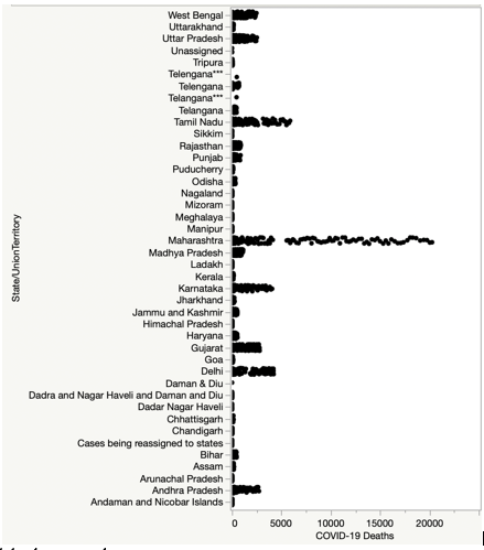
A visual display of the Kaggle-based first dataset is provided in Figure 1 for the first analysis model. The scatterplot shows variations between state/territory and COVID-19 caused deaths. It demonstrates that the state of Maharashtra has experienced more variation of deaths followed Tamil Nadu, Delhi, Karnataka, Gujarat, Andhra Pradesh, West Bengal, and Uttar Pradesh. The other states/territories have seen relatively lower deaths.

Figure 1

States and deaths scatterplot

Using JMP software, I performed a linear regression analysis for COVID-19 caused deaths as a dependent variable and states/territories as independent variable. The model’s summary of fit demonstrated an R-squared adjusted value of 0.3732. The analysis of variance of the full model is shown in Table 1. The overall model is significant with a p-value of <0.0001. This means that the regression model is better than just using a mean value to predict deaths. Table 2 shows that all individual sources of states/territories are significant with COVID-19 deaths as it has a p-value <0.0001. Analyzing for the p-values I conclude that most states/territories are significant to the regression model with a p-value <0.05. A few states/territories (Andhra Pradesh, Dadra Nagar Haveli, Daman and Diu, Haryana, Madhya Pradesh, Panjab, Rajasthan, Telangana, Uttar Pradesh, and Unassigned) are not significant to the regression model with p-value >0.05.

Table 1

ANOVA table – 1^st data set

Source	DF	Sum of Squares	Mean Square	F Ratio
Model	41	4543842139	110825418	78.4799
Error	5294	7475927678	1412151.1	Prob>F
C. Total	5335	1.202e+10		<0.0001

Table 2

Effect tests – 1^st data set

Source	DF	Sum of Squares	F Ratio	Prob>F
State/Territory	41	4543842139	78.4799	<0.0001

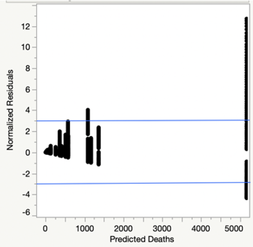
Figure 2 shows the normalized residuals vs. predicted deaths for the Kaggle data set 1 based model. There are many outliers when predicted deaths are higher than 5,000, as several of the points do not fall within a -3 to +3 range.

Figure 2

Normalized residuals plot

Second analysis model

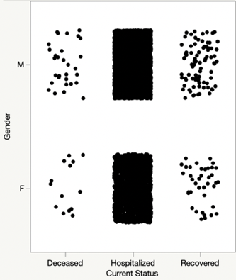
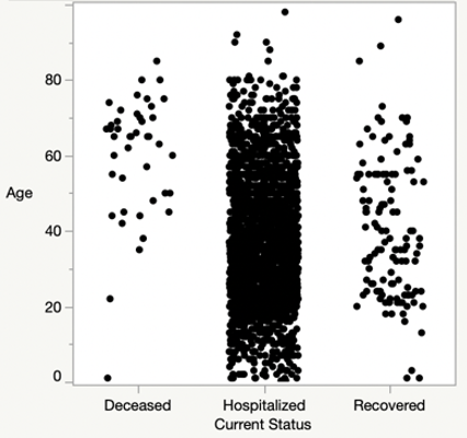
For the second model, multiple regression was performed using Kaggle’s second data set. The model included age, gender, states of residence, and count of COVID-19 deaths. A visual display of Kaggle-based second dataset is provided in Figure 3 through 6. These scatterplots show variations between gender and current status, age and current status, and states/territories and current status where current status takes a value of Deceased or Hospitalized or Recovered. Figure 3 demonstrates that both Males and Females experienced similar variations for each of the current status.

Figure 3

Gender and current status scatterplot

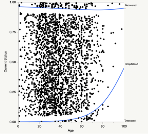
Figure 4 shows an increase in the number of deaths as a function of age. I reach the conclusion that if you are below the age of 40 your chance of death is very small while if you in the age group of 40 and above your chance of death is relatively higher. Most hospitalizations are for age of 70 and below while there are only few recoveries for the age over 70.

Figure 4

Age and current status scatterplot

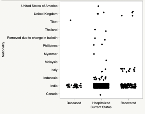
I have plotted nationality and current status related to COVID-19 based infections in Figure 5. It shows that Indian nationals are mostly affected on all fronts (diseased or hospitalized or recovered) compared to the foreign nationals being affected in the country.

Figure 5

Nationality and current status scatterplot

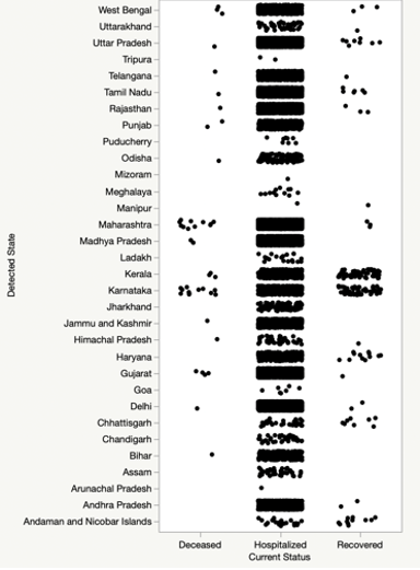
From Figure 6 , most states/territories have COVID-19 infected patients still hospitalized and in comparison the deaths are lot smaller in magnitude. The states of Kerala and Karnataka have most recovered patients than the other states in the country (diseased or hospitalized or recovered) compared to the foreign nationals being affected in the country.

Figure 6

States and current status scatterplot

I performed a multiple nominal logistics regression with current status as dependent variable y described by equation (4).Table 3 shows that the overall logistics regression model for the second Kaggle data set is significant with a p-value of <0.0001.

This means that the regression model is better than just using a mean value to predict deaths. The model had a R-squared value of 0.4105 Table 4 for this analysis demonstrated that age and states/territories of residence are statistically significant (p-value <0.05), however the gender is not statically significant with p-value of 0.0968 since it is greater than 0.05.

Table 3

Wholemodel test – 2^nd data set

Model	DF	-log likelihood	Chi Square	Prob>Chi Square
Difference	236	260	521	<0.0001
Full		374
Reduced		634

Table 4

Effect likelihood ratio tests – 2^nd data

Source	DF	L-R ChiSq	Prob>ChiSq
Age	174	248.3	<0.0002
Gender	2	4.7	0.0968
Detected State	60	260.7	<0.0001

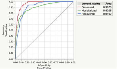
In Figure 7 I show the Receiver Operating Characteristics (ROC) plot for Kaggle’s second dataset which depicts sensitivity vs (1-specificity) for all three possibilities of current status due to virus infection. The area under the curve is the indicator of the goodness of fit for the model. A value of 1 indicating a perfect fit while value of 0.5 (represented by the diagonal in the figure) meaning that the model cannot discriminate among groups under consideration. Notice that all three curves have area values closer to 1 than 0.5 meaning a very good fit with the deceased group with the best fit out of all three options for the current status.

Figure 7

ROC plot

The second data set was run again for nominal logistics regression with this time age as the only independent variable and current status as a dependent variable. Figure 8 shows a logistics curve for this analysis. The lower curve in the plot shows the predictive probability of individual being diseased due to the virus depending on the age of the individual. The rising of the lower curve shows that higher the age higher the predictive probability of being diseased due to the virus. The upper curve shows the predictive probability of diseased or hospitalized individual on the basis of age. The distance between the two curves is the predictive probability of being hospitalized due to the virus depending on individual’s age. Thus higher the age relatively lower the predictive probability of being hospitalized compared to their younger counterparts. Notice also that the upper curve is flatter which means that combined predictive probability of diseased or hospitalized appears to be constant.

Figure 8

Logistics curve

Understanding Indian population

Table 5 depicts India’s top populated states with ranking based on urban population.12

I created Table 6 with the COVID-19 death rankings derived from Figure 1. I also added GDP rankings for the states for 2019-2020.13 COVID-19 deaths rankings for the states of residence match well with combination of urban population and GDP rankings. GDP creation requires people to interact with each other as close proximity realized in higher urban density setting would exacerbate the social distancing issues faced by the population.

Conclusions

India with 0.73% death rate would likely witness about 10M total deaths in 2020. If unchecked the death tally would include 200K-300K COVID-19 caused deaths. I observed that the states/territories of residence are a significant factor in the first regression model. The top 10 states experiencing COVID-19 deaths are found to be in top 10 urban population ranked states coupled with top 15 GDP creation. Case in point are Maharashtra with urban population rank 1^st and GDP rank 1^st had highest COVID-19 caused deaths in the country and the state of Tamil Nadu with urban population rank of 3^rd and GDP rank of 2^nd had the second highest COVID-19 deaths. Forced avoidance of social distancing in larger urban and high GDP creating states may be the driver in getting higher COVID-19 infections and deaths.

Factors of age, and state of residence were found statistically significant using logistical regression analysis, however, gender was found to be not statistically significant. The data thus shows that virus does not spare any gender over other and is equal opportunist as it kills both genders equally. The age is a critical variable that decides death over life and is pronounced especially for population over age of 40.

As the younger population less than age of 30 is spared by the virus may point to opening face-to-face academic learning. Focusing on 200K-300K likely deaths due to COVID-19 in 2020 misses the remaining bigger picture of 10M annual deaths caused by other issues in the society.

Acknowledgments

None.

Source of Funding

No financial support was received for the work within this manuscript.

Conflicts of Interests

None.